A Brief Introduction to Dimensionality Reduction: PCA and t-SNE

In machine learning, having too many features can lead to several problems, such as:

• Overfitting
• Slower processing speeds
• Difficulty visualizing data with more than three features

This is why dimensionality reduction becomes necessary. In practice, when dealing with hundreds or thousands of features, manually picking them is clearly not a sensible approach. Below, we introduce two widely used dimensionality reduction techniques in machine learning.

PCA (Principal Component Analysis)

Before introducing PCA, let’s first define our objective:

Transform a sample from an n-dimensional feature space into a k-dimensional feature space, where k < n.

Here are the main steps of PCA:

1. Standardize the data
2. Construct the covariance matrix
3. Use Singular Value Decomposition (SVD) to obtain the eigenvectors and eigenvalues
4. Sort the eigenvalues in descending order and select the top $k$ eigenvalues and their corresponding eigenvectors
5. Project (map) the original data onto the eigenvectors to obtain the new set of features

The most crucial component of PCA is Singular Value Decomposition. Therefore, let’s take a closer look at SVD in the next section.

Intuitive Understanding of Singular Value Decomposition

In matrix factorization, Singular Value Decomposition is a well-known method. In high school mathematics, the most common application of matrix factorization is solving systems of equations (such as LU decomposition). We can gain an intuitive understanding from the SVD formula:

Where $A$ is an $m \times n$ matrix, $U$ and $V$ are orthogonal matrices, and $\Sigma$ is the singular value matrix. The singular values correspond to the eigenvalues of matrix $A$. In PCA, these are also referred to as principal components, representing the importance of the preserved information. They are arranged in descending order along the diagonal, forming a diagonal matrix.

So what does $A$ correspond to here? Naturally, it corresponds to our features. However, it is important to note that here, we usually compute $A$ using the covariance matrix. Remember that the data must be standardized before performing SVD.

Covariance matrix

Because the covariance matrix is often denoted by Sigma, make sure not to confuse it with $\Sigma$ above. To reduce dimensions, we can multiply the first $k$ columns of $U$ by the corresponding singular values in $\Sigma$ to obtain the new features. From a geometric perspective:

Geometrically, this operation actually projects $X$ onto the first $k$ vectors of $U$.

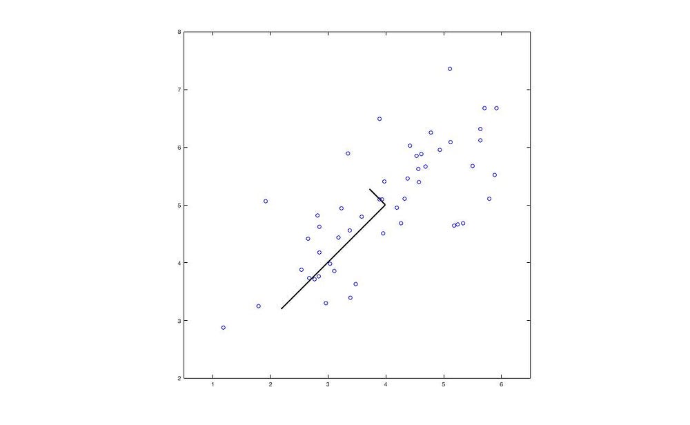
The black line represents the eigenvector, and its length corresponds to the eigenvalue.

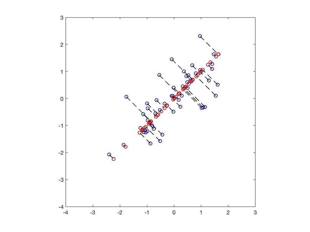
The blue dots represent the original positions of the data, while the red dots represent their projected positions on the eigenvector. With this, we have successfully reduced 2D data down to 1D.

Naturally, we can also reduce from 3D to 2D:

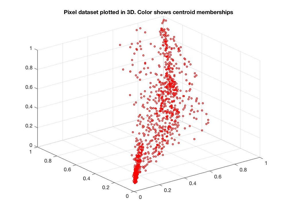
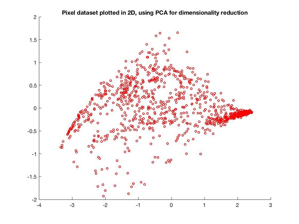
Applications of PCA

During dimensionality reduction, we want to retain the most critical features and discard the less important ones.

For example, when recognizing a person, the most important identifying features might be the eyes, nose, mouth, etc., whereas features like skin tone or hair can be discarded. In fact, PCA is commonly used for dimensionality reduction in facial recognition (Eigenfaces).

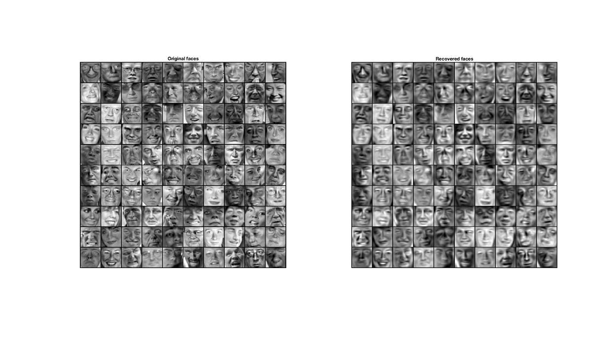
This provides an intuitive overview of SVD. Due to length constraints, we cannot dive deeply into every detail. If you are interested in SVD, feel free to check out Wikipedia.

t-SNE

PCA is an intuitive and effective dimensionality reduction technique. However, as seen when converting from 3D to 2D, some clusters can end up completely jumbled together.

PCA is a linear dimensionality reduction method. If the relationships between features are nonlinear, using PCA may lead to underfitting.

t-SNE is another dimensionality reduction technique, but it uses a more sophisticated approach to model relationships between high-dimensional and low-dimensional spaces. t-SNE approximates high-dimensional data using the probability density function of a Gaussian distribution, while using a Student’s t-distribution to approximate the low-dimensional data. It then computes similarities using Kullback-Leibler (KL) divergence and optimizes via gradient descent (or stochastic gradient descent).

Probability Density Function of the Gaussian Distribution

Where $X$ is a random variable, $\sigma$ is variance, and $\mu$ is the mean.

Thus, the original high-dimensional data can be expressed as:

And the low-dimensional data can be represented using the probability density function of a Student’s t-distribution (with 1 degree of freedom):

Where $x$ represents data points in high-dimensional space, and $y$ represents data points in low-dimensional space. $P$ and $Q$ denote their respective probability distributions.

Why use a Student’s t-distribution to approximate low-dimensional data? Mainly because projecting down to lower dimensions inevitably causes significant information loss. A t-distribution prevents the projection from being overly affected by outliers.

When sample sizes are small, the t-distribution models the population distribution better and is less sensitive to outliers.

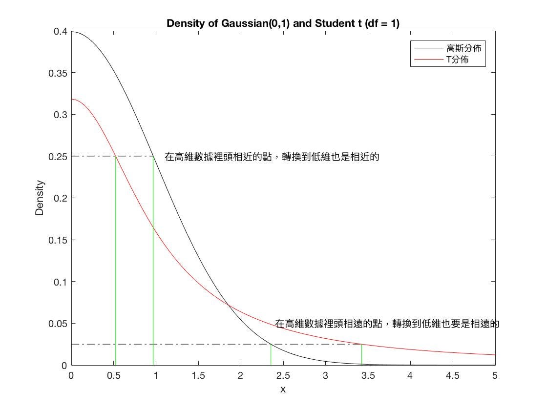Probability density functions of the Student’s t-distribution and Gaussian distribution

Similarity Between Two Distributions

To calculate the similarity between two distributions, KL divergence (Kullback-Leibler Divergence) is commonly used, also known as Relative Entropy.

t-SNE uses perplexity (Perp) as a hyperparameter.

The original paper states that perplexity is typically chosen between 5 and 50.

Cost Function

Calculating Cost using KL divergence:

Computing the gradient yields:

Finally, gradient descent (or stochastic gradient descent) is used to find the minimum.

Practical Experiment: Testing on MNIST

The test dataset can be downloaded here. First, let’s look at the result when reducing to 2D using PCA.

PCA

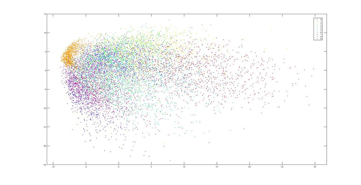PCA Dimensionality Reduction

As you can see, after reducing down to 2D, the data is jumbled together into a single mass with virtually indistinguishable clusters. This happens because PCA’s linear projection loses too much information along the way.

t-SNE

Next, let’s test with t-SNE:

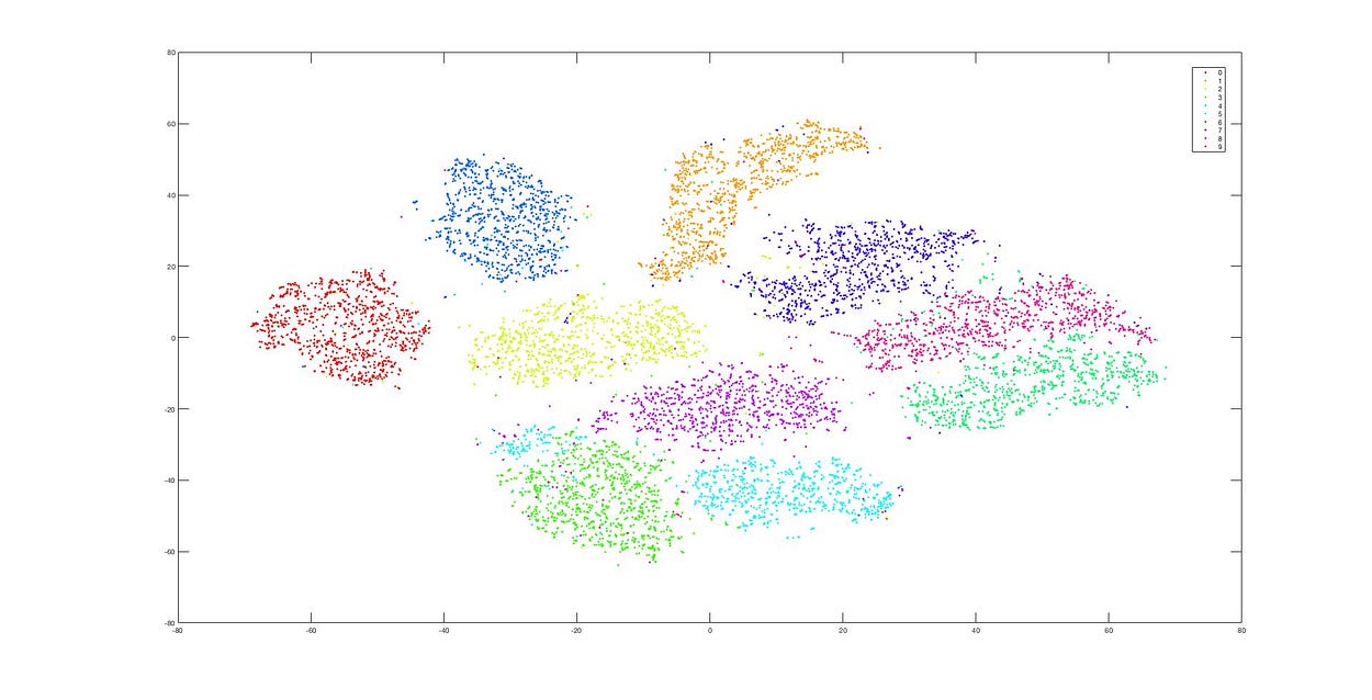Dimensionality Reduction with t-SNE

This is the result using t-SNE. Even after dimensionality reduction, the data remains cleanly clustered. The difference between the two (PCA vs. t-SNE) is strikingly evident across these two figures.

Summary

Subsequently, several algorithms were proposed to enhance the performance of t-SNE; for details, see Accelerating t-sne using tree-based algorithms. Most popular data analysis languages and libraries have implemented it, including scikit-learn, R, MATLAB, and others.

However, because t-SNE is a nonlinear dimensionality reduction method, its execution time is significantly longer than that of PCA.

• When there are too many features, using PCA might cause the reduced features to underfit; in such cases, consider using t-SNE instead.
• t-SNE requires noticeably more computational time.
• The paper also describes several optimization techniques (such as how to choose perplexity). Since I haven’t finished reading it all yet, I will update this post with more details in the future.

References

• Van der Maaten L, Hinton G. Visualizing data using t-SNE
• Accelerating t-sne using tree-based algorithms Accelerating t-SNE computation using various tree-based algorithms
• 線代啟示錄 - 奇異值分解

This article was also published on Medium