Talking about PCA and T-Sne in Reduction Methods

In machine learning, having too many features can lead to several issues, such as:

• Overfitting
• Slower processing speed
• Difficulty visualizing if there are more than three features

This is when dimensionality reduction becomes necessary. In practice, manually selecting features from hundreds or thousands is clearly not a wise approach. Therefore, we will introduce two commonly used dimensionality reduction methods in machine learning.

PCA (Principal Component Analysis)

Before we dive into PCA, let’s define our objective:

Transform a sample with n feature space into a sample with k feature space, where k < n.

Here are the main steps of PCA:

1. Standardize the data
2. Create a covariance matrix
3. Use Singular Value Decomposition (SVD) to find the eigenvectors and eigenvalues
4. Usually, eigenvalues are arranged in descending order, and we select the top k eigenvalues and their corresponding eigenvectors
5. Project the original data onto the eigenvectors to obtain new features

The most crucial part of PCA is the Singular Value Decomposition, so let’s discuss SVD in the next section.

Intuitive Understanding of Singular Value Decomposition

Among matrix decomposition methods, Singular Value Decomposition is quite well-known. The most common use of matrix decomposition in high school mathematics is solving equations (like LU decomposition). From the formula of SVD, we can intuitively understand:

Where A is an m x n matrix, 𝑈 and V are orthogonal matrices, and 𝛴 is the singular value matrix. The singular value matrix corresponds to the eigenvalues of matrix A, known as principal components in PCA, which indicate the importance of retaining information, usually arranged in descending order along the diagonal, forming a symmetric matrix.

So what does A correspond to here? It corresponds to our features, but it’s particularly important to note that we typically compute A using the covariance matrix. Remember, the data must be normalized before performing Singular Value Decomposition.

Covariance matrix

The covariance matrix is often represented by Sigma, so don’t confuse it with the 𝛴 above. Therefore, to reduce dimensions, we can multiply the first k rows of U with the corresponding eigenvalues in 𝛴 to obtain new features; geometrically speaking,

This operation in geometry is essentially projecting X onto the first k vectors of U.

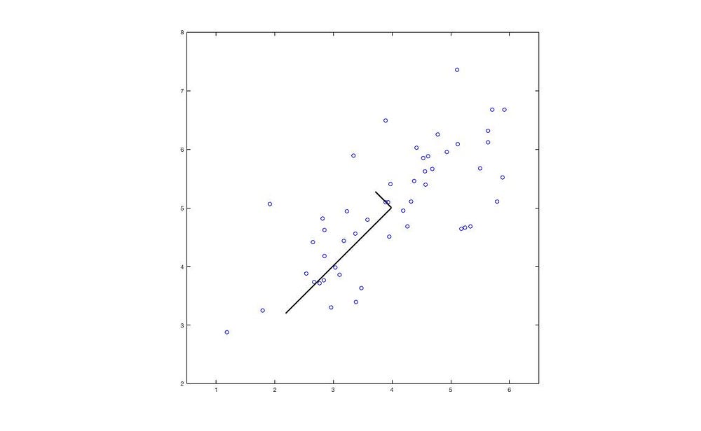
The black lines represent the eigenvectors, with lengths corresponding to the eigenvalues.

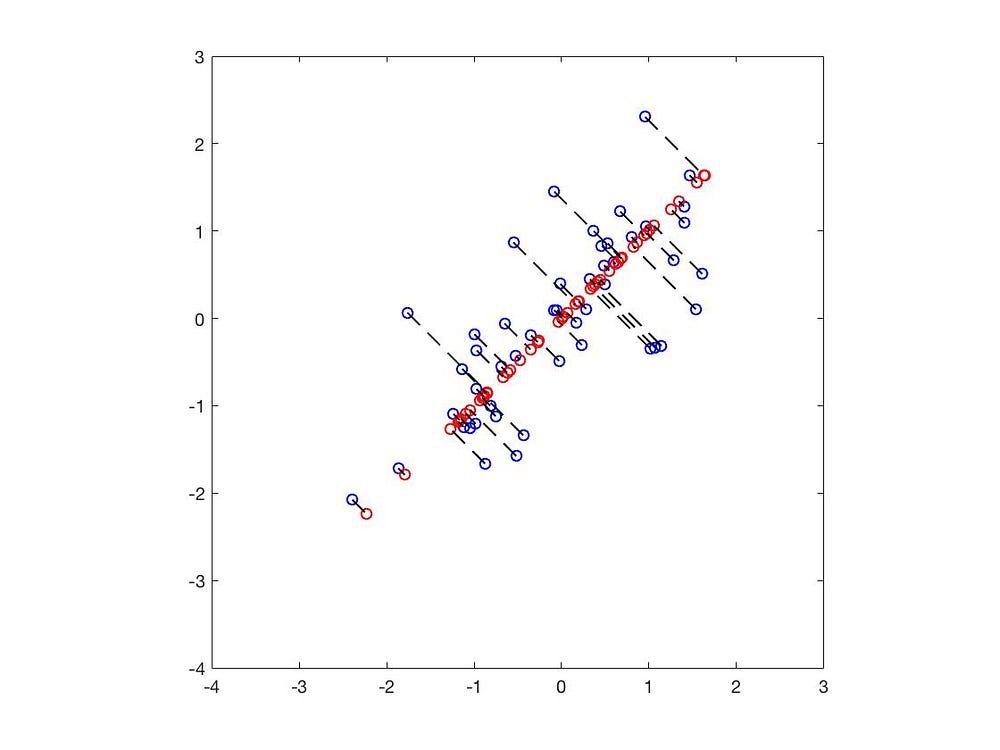
The blue dots represent the original data points, while the red dots indicate the positions projected onto the eigenvectors. Thus, we have successfully reduced the 2D data to 1D.

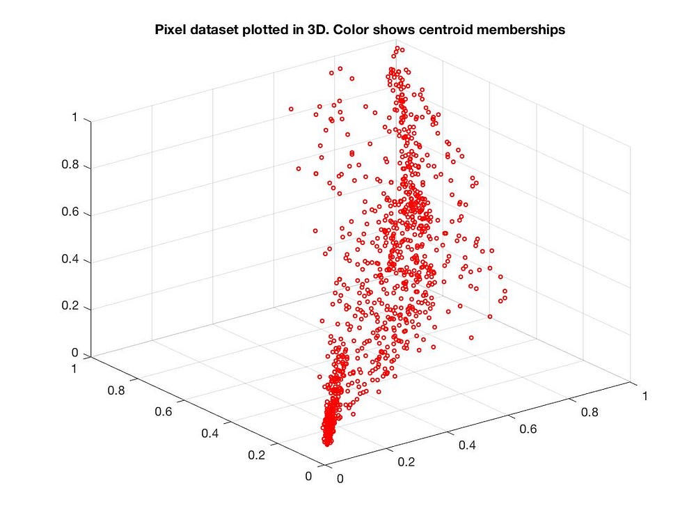
We can also reduce from 3D to 2D:

Applications of PCA

When performing dimensionality reduction, we aim to retain the most important features, discarding the less significant ones.

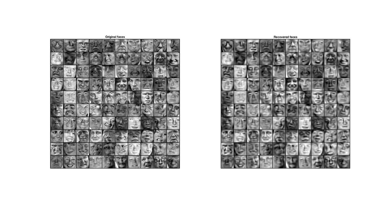
For instance, when judging a person, the most critical distinguishing features may be the eyes, nose, and mouth, so we can discard features like skin color and hair. In fact, PCA is often utilized for dimensionality reduction in facial recognition.

This provides an intuitive understanding of Singular Value Decomposition. Due to space constraints, we cannot delve deeper into the topic. If you're interested in SVD, feel free to check out Wikipedia.

t-SNE

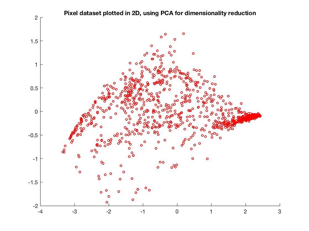
PCA is a fairly intuitive and effective dimensionality reduction technique. However, when transitioning from three dimensions to two, we can see that some data clusters become completely jumbled.

PCA is a linear dimensionality reduction method, but if the relationships between features are nonlinear, using PCA might lead to underfitting.

t-SNE is another dimensionality reduction technique, but it employs more complex formulas to express the relationship between high-dimensional and low-dimensional data. t-SNE primarily approximates high-dimensional data using a Gaussian distribution probability density function, while the low-dimensional data is approximated using a t-distribution. It calculates similarity using KL divergence and ultimately finds the optimal solution through gradient descent (or stochastic gradient descent).

Gaussian Distribution Probability Density Function

Here, X is the random variable, 𝝈 is the variance, and 𝜇 is the mean.

Thus, the original high-dimensional data can be represented as:

And the low-dimensional data can be represented using the t-distribution probability density function (with 1 degree of freedom):

Where x represents the data in high-dimensional space, and y represents the data in low-dimensional space. P and Q represent the probability distributions.

Why use a t-distribution to approximate low-dimensional data? The main reason is that transitioning to a lower dimension will inevitably result in the loss of significant information. To avoid being influenced by outliers, the t-distribution is used.

The t-distribution can better model the population distribution when the sample size is small and is less influenced by outliers.

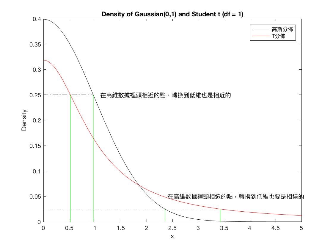T-distribution vs. Gaussian distribution probability density functions

Similarity Between Two Distributions

To calculate the similarity between two distributions, KL divergence (Kullback-Leibler Divergence) is often used, also known as relative entropy.

In t-SNE, perplexity (Perp) is used as a hyperparameter.

The paper suggests that perplexity typically ranges from 5 to 50.

Cost Function

The cost is computed using KL divergence.

The gradient can be expressed as:

Finally, using gradient descent (or stochastic gradient descent), we can find the minimum value.

Experiment: Testing with MNIST

You can download the test set here. First, let's reduce the dimensions to two using PCA.

PCA

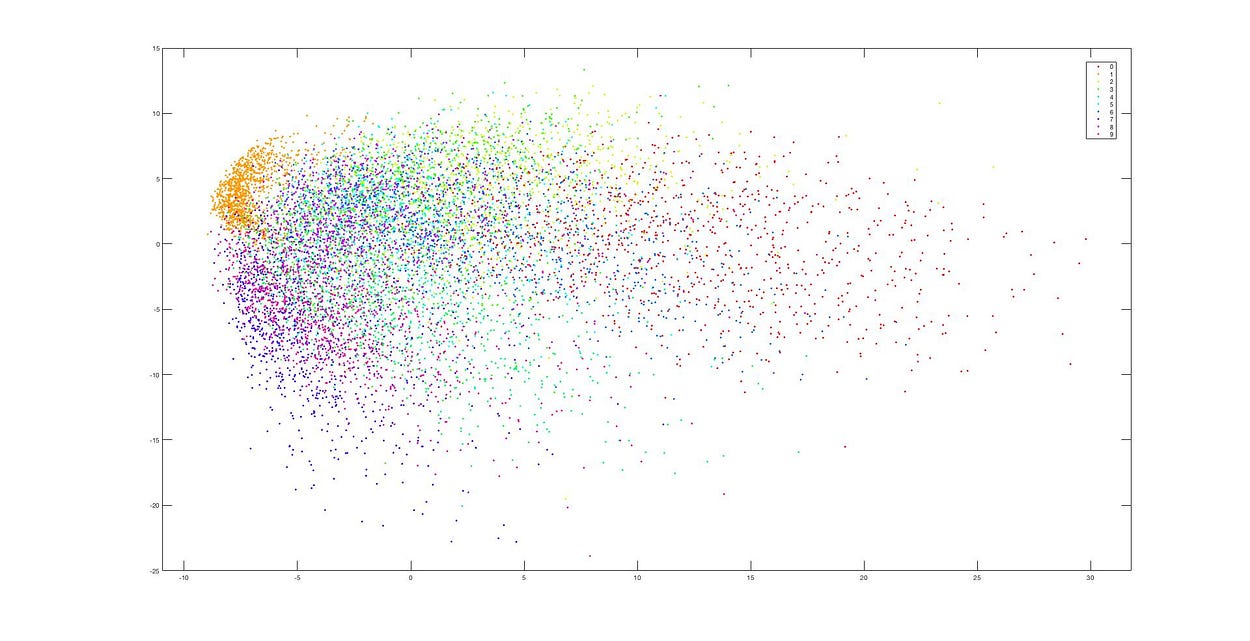PCA Dimensionality Reduction

We can see that after reducing to two dimensions, the data appears almost jumbled together, making it impossible to discern clusters. This is because PCA's linear dimensionality reduction loses too much information in the process.

t-SNE

Next, we will test using t-SNE.

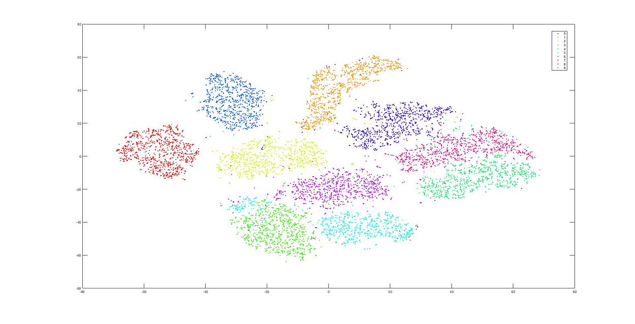Dimensionality Reduction using t-SNE

This is the dimensionality reduction result after using t-SNE, and we can see that the data clusters remain distinct. The difference between these two methods (PCA and t-SNE) is quite evident from these images.

Summary

Subsequently, a series of algorithms were proposed to improve the performance of t-SNE. For more details, refer to Accelerating t-SNE using tree-based algorithms. Most popular data analysis programming languages, such as sklearn, R, and MATLAB, have also implemented these methods.

However, t-SNE is not a linear dimensionality reduction method and will generally take much longer to execute compared to PCA.

• When the number of features is too high, using PCA may lead to underfitting in the reduced features; at this point, consider using t-SNE for dimensionality reduction.
• t-SNE requires significantly more execution time.
• The paper also includes optimization techniques (such as how to choose perplexity, etc.). Since I haven't finished reading it yet, I will gradually add more information later.

References

• Van der Maaten L, Hinton G. Visualizing data using t-SNE
• Accelerating t-SNE using tree-based algorithms Using various tree algorithms to accelerate t-SNE computations
• Linear Algebra Revelation - Singular Value Decomposition

This article is also published on Medium.